Frequently, the geologist does the initial logging of wells and the hydrologist or hydrogeologist interprets these logs into a coarser aggregation that lumps together the fine-scaled designations applied by the geologist. This interpreted geology is referred to as stratigraphy and is plotted as Fence Diagrams or Geologic Models.
Three-dimensional models can be constructed in EnviroInsite as either open like a 3D fence diagram or closed to attain the visual appearance of a solid object. Both types of plots are generated by selecting Plot> Stratigraphy> Model from the main menu. There are two options, "Auto-generated Line" and "Manual". Auto-generated Line will automatically create a closed stratigraphy plot surrounding the selected locations at the defined radius. The Manual option will prompt users to draw a polyline along which the 3D geologic model will be constructed. By electing to create a closed polygon, a 3D solid object is created. Fence diagrams and 3D geologic models are generated by interpolation of the contact elevation to the defining polygon. The vertical areas are then filled. For the case of a closed polygon, the surface is drawn by interpolating the contact elevation surface onto a regular grid.
View a training video on modeling of Stratigraphy here.
Manual 3D Stratigraphy Model
Follow these steps to create a manual 3D stratigraphic model:
1.Plot locations in Plan View.
2.From the main menu, click Plot> Stratigraphy> Model > Manual.
3.Use the left mouse button to click points within the map to define the model area.
4.To complete the selection, double-click or right-click with the mouse on the last point in the model.
5.The 3D Stratigraphy dialog box opens. Modify the model properties on all tabs (Query, Format, Interpolation, and EQuIS Location Groups) as desired. Click the OK button to save changes.
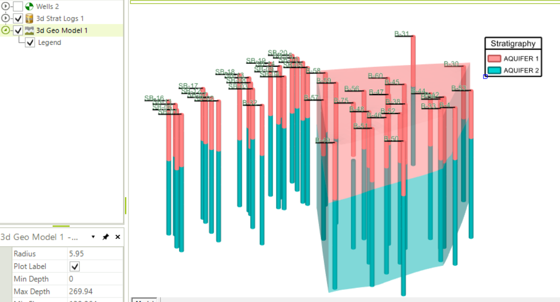
Auto-generated Line 3D Stratigraphy Model
The auto-generated line 3D stratigraphy model automatically draws polylines around the selected locations by connecting each location to the closest location using the specified radius.
Example
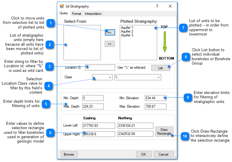
Query Tab
The query dialog box is similar to that used in other parts of the application. In this case, select the stratigraphic units to be plotted. Select units from the list box on the left and click the => button to include them in the list of units to be plotted. The units should be in order from top-down of their appearance in the physical model. That is, the uppermost units in the real world should be added to the list first followed by the other units.
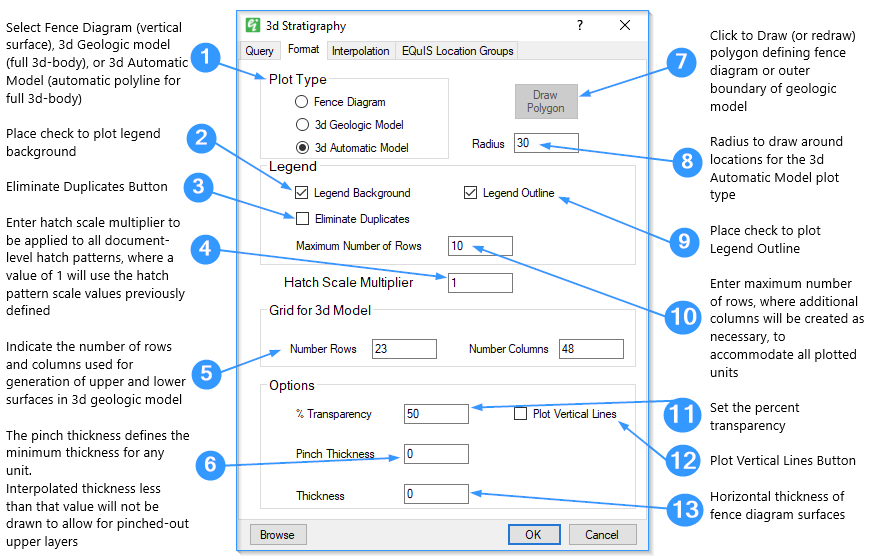
Format Tab
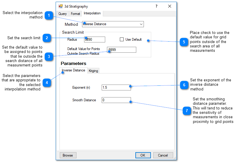
Interpolation Tab
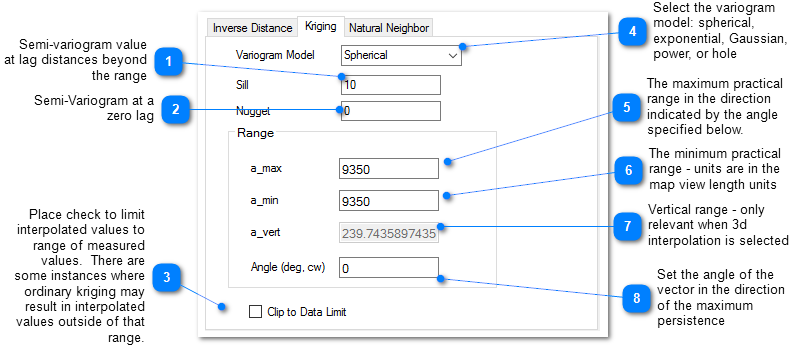
This tab allows the user to select the interpolation scheme and the parameters of the interpolation method. The correct selection of interpolation parameters is critical to generate contours that accurately reflect the field data and our expectations of how the values vary between the measured data points. The default parameters are frequently adequate, although some improvement can be anticipated through trial and error. There is no single, objectively optimal set of interpolation parameters. Different methods and parameters work best for different data sets.
Kriging Parameters
The kriging routines are derived from the kt3d routine of the Geostatistical Software Library (GSLIB) authored by Clayton Deutsch and Andre Journel.
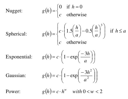
The reference GSLIB: Geostatistical Software Library and Users' Guide is highly recommended. The following equations are the spherical semivariogram models used by EnviroInsite for an isotropic system, where h is the lag, c is the sill, and a is the (practical) range.
(Source: Introduction to Geostatistics and Variogram Analysis, available here).
For anisotropic systems, h/a in the previous is calculated as
![]()
Inverse Distance Parameters
Exponent – The measured values are assigned weights that are equal to one over the distance between the measured value and the grid point raised to some power. This exponent is the power used in that calculation.
Smooth Distance – The inverse distance method tends to cause a kind of bubbly surface with the bubbles coinciding with measurement points. This type of trend can be reduced by introducing a non-zero smoothing distance. The smoothing distance is effected by adding this distance to the separation distance between the measurement point and the grid point prior to calculating the interpolation weight. This effectively diminishes the weight assigned to points at distances close to the Smooth-Distance, while not appreciably impacting the calculated weights for more distant points.