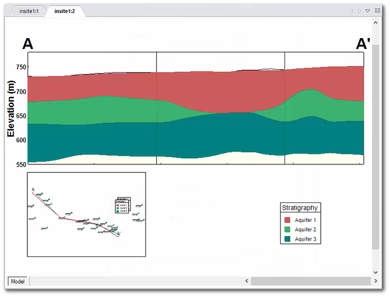
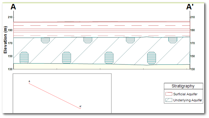
Frequently, the geologist does the initial logging of wells and the hydrologist or hydrogeologist interprets these logs into a coarser aggregation that lumps together the fine-scaled designations applied by the geologist. This interpreted geology is referred to as stratigraphy and is plotted as Fence Diagrams or Geologic Models. Geologic models may also be plotted on cross-sections, as in the following image.
Once the cross-section is created using the steps listed in the Cross-Section Trace help page, the stratigraphy model can be drawn by selecting Plot > Stratigraphy > Model from the main menu.
For EQuIS databases, Stratigraphy models on the cross-section are drawn based on the records in the DT_LITHOLOGY table. Additional information is available here in the EQuIS Data Tables and Field help page.
For EnviroInsite databases, stratigraphy models on the cross-section are drawn based on the records in the Stratigraphy table. The resulting model may be edited manually by selecting individual points on the contact surface and then dragging the points upward or downward. To preserve these manual edits, select the Detach from Data option of the Profile Stratigraphy plot object.
To create a 3D model, click Plot> Stratigraphy from the main menu and select Model. The Profile Stratigraphy dialog box opens. Modify the model properties on the Query tab, Format tab, Interpolation tab, and EQuIS Location Groups tab as desired. Click the OK button to save changes.
Query Tab
The query dialog box is similar to that used in other parts of the application. In this case, select the stratigraphic units to be plotted. Select units in the Select From list box on the left and click the => button to include them in the list of units to be plotted (i.e., Plotted Stratigraphy list box). The units should be in top-down order of their appearance in the physical model. That is, the uppermost units in the real world should be added to the list first followed by the other units.
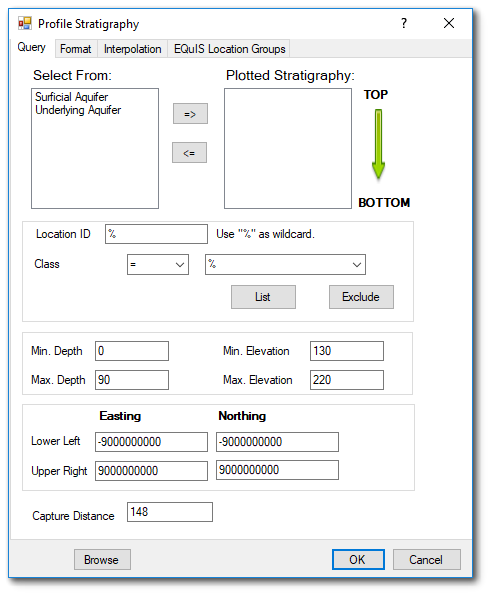
Location ID – Enter string to filter by Location ID, where "%" is used as a wild card.
Class – Use the drop-down menu to select Location.Class value to filter this field's content.
Depth and Elevation – Set the minimum and maximum depth limits and elevation limits for filtering of stratigraphic units.
Selection Rectangle – Enter easting and northing values to define the selection rectangle used to filter boreholes that will generate geologic model.
Capture Distance – Specify the maximum distance from the profile-defining polyline for which the stratigraphy values will be queried.
Format Tab
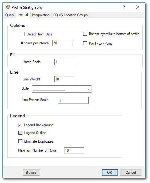
Options
Detach from Data – Check to not use database for determining how stratigraphic units are drawn. This is automatically selected following the editing of stratigraphic unit contact surfaces.
Bottom Layer Fill – Check to extend model to bottom of profile. This may be useful where the borehole depths are not sufficient to ascertain the bottom depth of the deepest stratigraphic unit.
Points per Interval – Set the number of points per interval for which the surfaces will be interpolated.
Point-to-Point – Check to draw stratigraphy using straight lines between units within the profile capture distance. This option will not use interpolation, which may result in the appearance of mis-specified unit heights for off-profile boreholes.
Fill
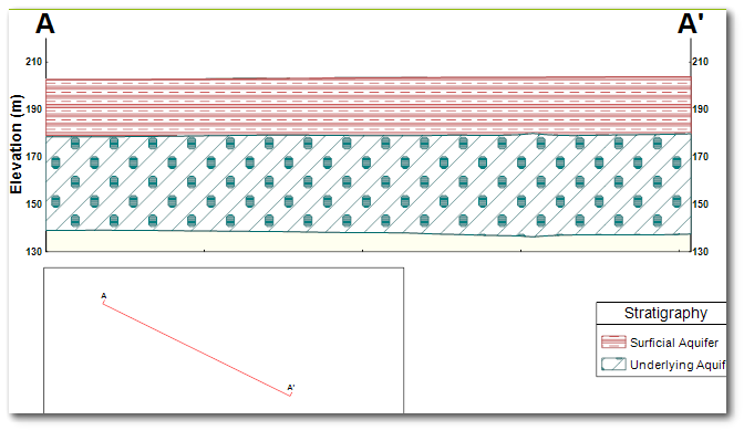
Hatch Scale – The hatch scale multiplier is applied to the hatch scale value for all stratigraphy elements of the current object. The default hatch scale is defined at a document level and may be modified by selecting Edit> Format> Stratigraphy from the main EnviroInsite menu. The following example illustrates how the hatch scale can impact the appearance of the stratigraphic style.
|
|
Stratigraphy with Original Hatch Scale |
Stratigraphy with Hatch Scale of 0.25 |
Line
Weight – Set the line weight in 100ths of mm.
Style – Use the drop-down menu to select the line style.
Legend
Background – Check to plot legend background.
Outline – Check to plot legend outline.
Eliminate Duplicates – Check to eliminate duplicates in legend.
Maximum Number of Rows – Enter the maximum number of rows, where additional columns will be created as necessary to accommodate all plotted stratigraphic units.
Interpolation Tab
This tab allows the user to select the interpolation scheme and the parameters of the interpolation method. Selection of interpolation parameters is critical to generate contours that accurately reflect the field data and our expectations of values between the data points. The default parameters are generally adequate, although some improvement can be anticipated through trial and error. There is no single, objectively optimal set of interpolation parameters. Different methods and parameters work best for different data sets.
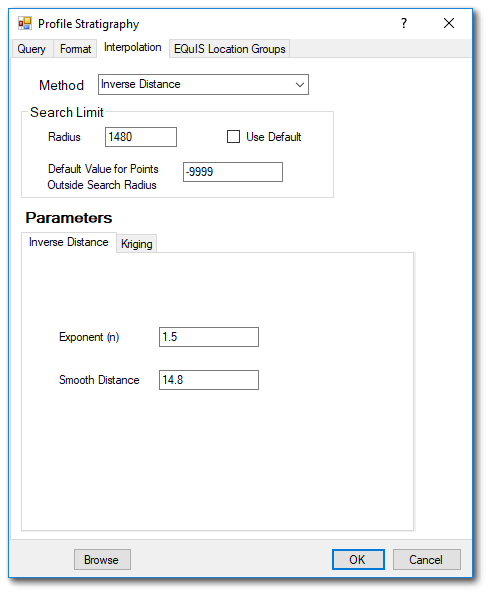
Method – Use the drop-down menu to select the contouring method, either inverse distance or kriging.
Search Limit
Radius – The cutoff distance establishes the maximum distance from the interpolated point for which a measured value will be used in the interpolation function. Used by both kriging and inverse distance routines.
Default Value for Points Outside Search Radius – This is the default value for points within the grid that are interpolated because they lie outside the search radius.
Use Default – Specify whether or not to use the default value. If not checked, then the non-interpolated nodes will not be contoured.
Inverse Distance Parameters
Exponent – The measured values are assigned weights that are equal to one over the distance between the measured value and the grid point raised to some power. This exponent is the power used in that calculation.
Smooth Distance – The inverse distance method tends to cause a kind of bubbly surface with the bubbles coinciding with measurement points. This type of trend can be reduced by introducing a non-zero smoothing distance. The smoothing distance is effected by adding this distance to the separation distance between the measurement point and the grid point prior to calculating the interpolation weight.
Kriging Parameters
The kriging routines are derived from the kt3d routine of the Geostatistical Software Library (GSLIB) authored by Clayton Deutsch and Andre Journel.
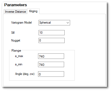
Variogram Model – Use the drop-down menu to select the variogram model. Choose from the spherical, exponential, gaussian, power, and hole variogram models using conventions of GSLIB.
Sill – Set the variogram model sill or c value.
Nugget – Set the local scale variability.
Range a_max – Set the maximum horizontal range.
Range a_min – Set the minimum horizontal range.
Angle – The rotation angle (in degrees clockwise about 12 o'clock) of axis defining the direction of maximum horizontal range. In some cases, it may be advantageous to increase the a_max value and to align this axis with the direction of groundwater flow.
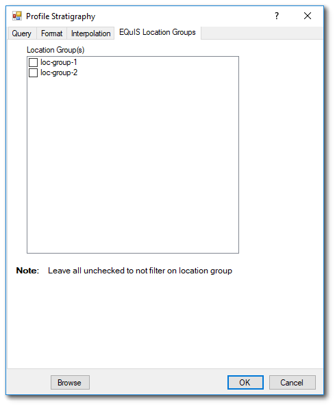
EQuIS Location Group Tab
If desired, check location groups.