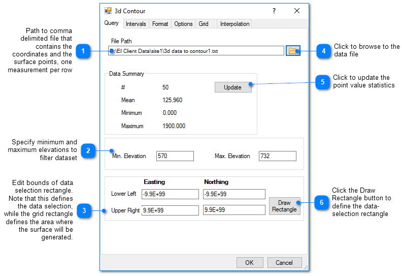
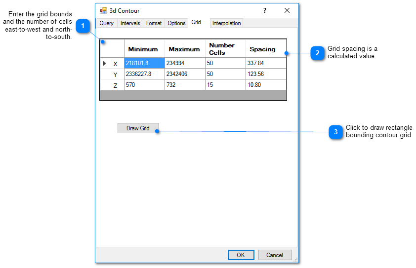
This contour-points routine generates 3D contours or 2D-profile contours from point data stored in text files. Each record has the X-Y-Z coordinates and a data value. The files can be comma-delimited or space-delimited. The control options are the same as the 3D contour options used in contouring measured data from a database.
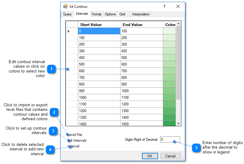
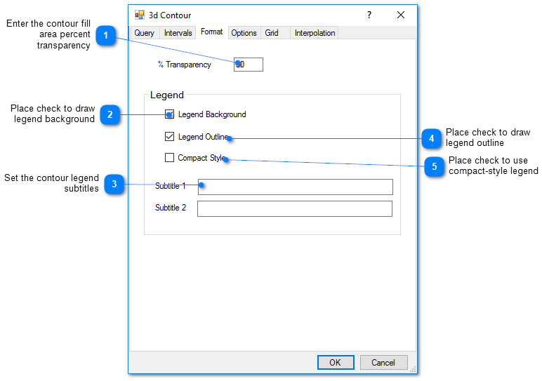
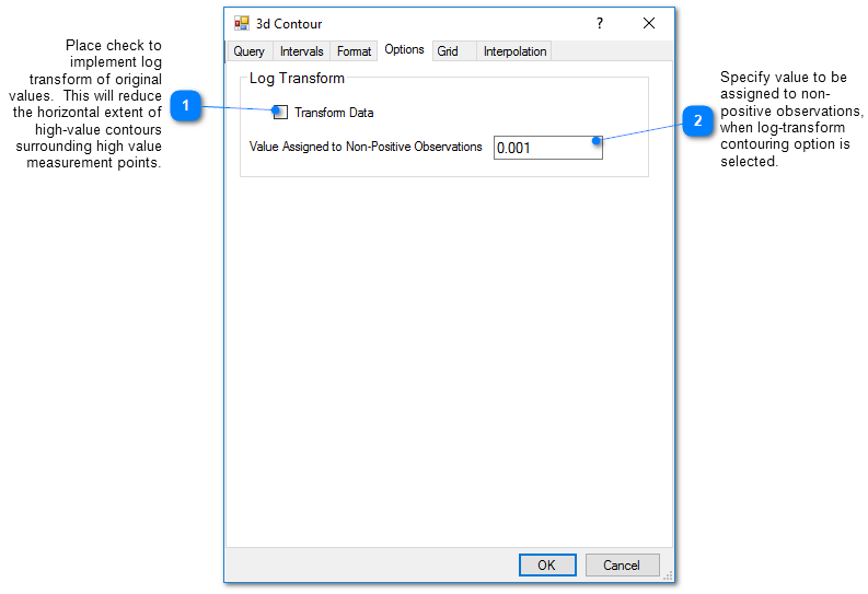
To create a 3D contour using external data, click Plot> External Data from the main menu and select 3D Contour. The 3D Contour dialog box opens. Modify the contour properties on the following tabs as desired:
Click the OK button to save changes.
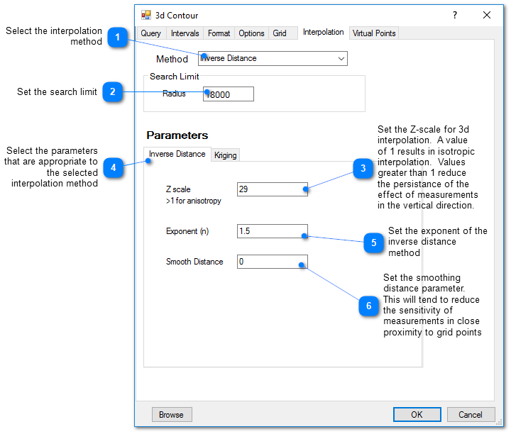
This tab allows the user to select the interpolation scheme and the parameters of the interpolation method. The correct selection of interpolation parameters is critical to generate contours that accurately reflect the field data and our expectations of how the values vary between the measured data points. The default parameters are frequently adequate, although some improvement can be anticipated through trial and error. There is no single, objectively optimal set of interpolation parameters. Different methods and parameters work best for different data sets.
Kriging Parameter
The kriging routines are derived from the kt3d routine of the Geostatistical Software Library (GSLIB) authored by Clayton Deutsch and Andre Journel.
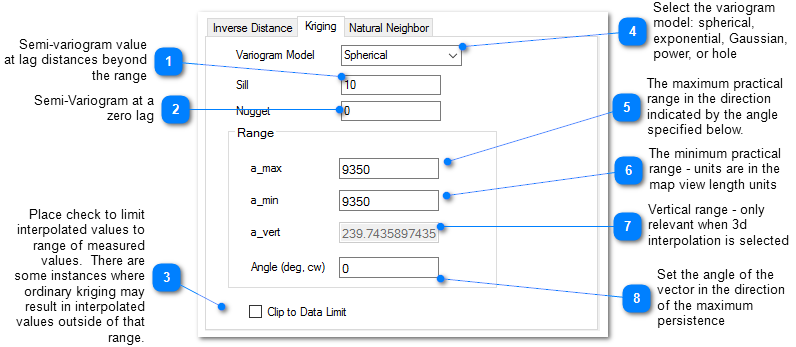
The reference GSLIB: Geostatistical Software Library and Users' Guide is highly recommended. The following equations are the spherical semivariogram models used by EnviroInsite for an isotropic system, where h is the lag, c is the sill, and a is the (practical) range.
(Source: Introduction to Geostatistics and Variogram Analysis, available here).
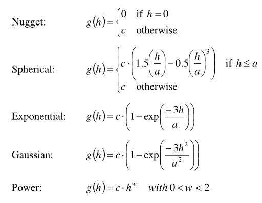
For anisotrophic systems, h/a in the previous is calculated as
![]()