Generation of 3D contours within EnviroInsite is an internal three-step process. The data are queried to select the set of measurements for which the contours will be constructed. Then the measured data is interpolated on the corners of a 3D mesh. Lastly, surfaces are generated representing the selected contour intervals.
The 3D mesh is rectangular, with its lateral extent, vertical extent, and horizontal and vertical discretization selected by the user. A finer mesh will create a smoother surface, but may be time consuming to create. There are no absolute constraints as to the number of grid points other than the physical memory in the computer. In most practical cases, the time to plot and the physical memory will not be significant constraints.
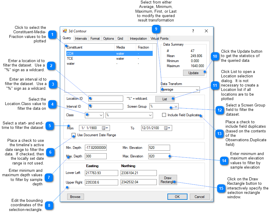
Click Plot> 3D Data from the main menu and select Contours. The 3D Contour dialog box opens. Modify the contour properties on the Query tab, Interval tab, Format tab, Options tab, Grid tab, Interpolation tab, Virtual Points tab, and EQuIS Query tab as desired. Click the OK button to save changes.
Query Tab
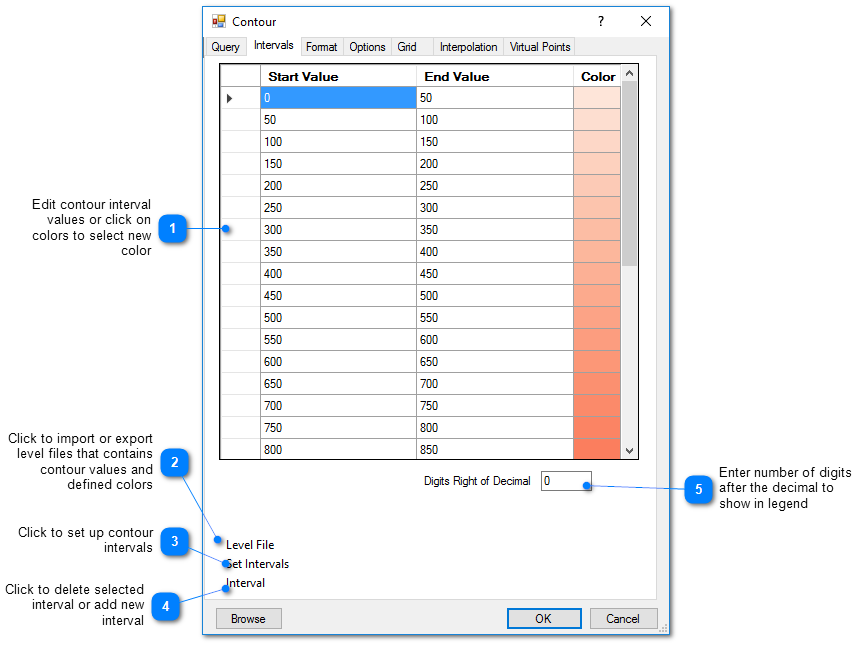
Intervals Tab
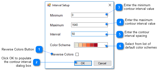
Interval Setup
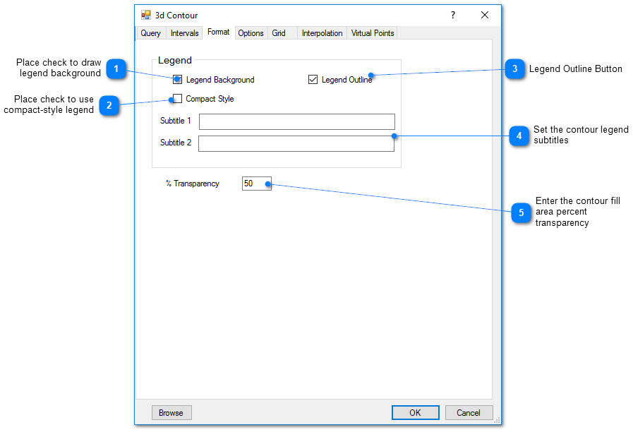
Format Tab
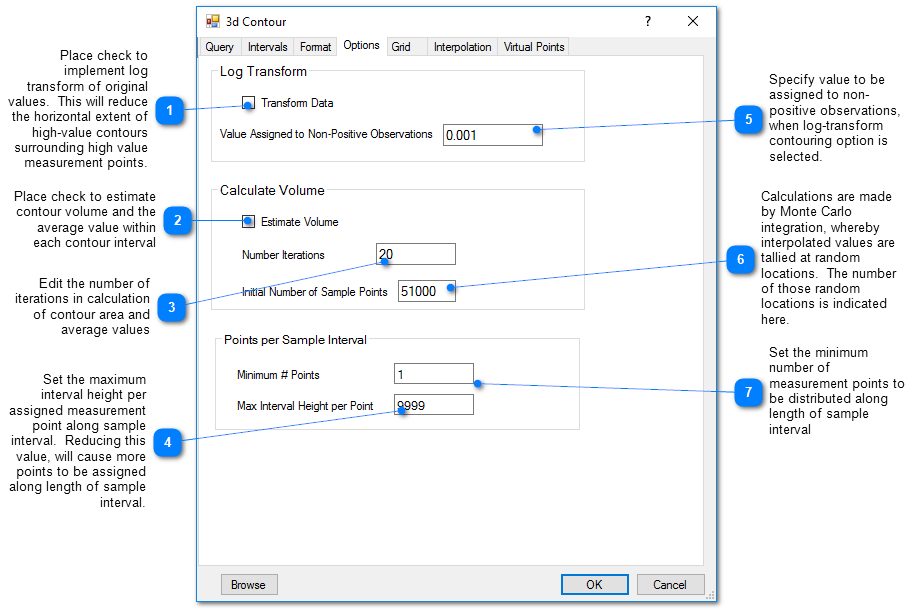
Options Tab
3D Contour Option
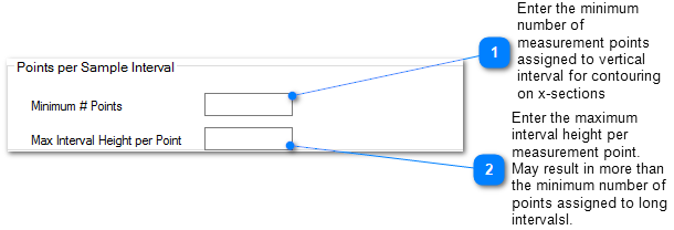
In 3D contouring, multiple measurement points are assigned along the length of the specified measurement interval. The first value in the Points per Sample Interval is the minimum number of points that are assigned to a sample interval. Then the interval height per measurement point is calculated. If this exceeds the entered Max Interval Height per Point, the number of points to achieve that value is calculated and that number of points is distributed along the interval horizon.
3D Contour Volume Calculation
For 3D contouring, EnviroInsite can estimate the volume occupied by each contour interval and the average value within that interval. The calculations are performed by interpolation to randomly sampled points within the contour grid and estimation of the average interpolated value within each contour interval. The occupied volume is estimated as the grid volume and the fraction of the sample points with values within a given contour interval relative to the total number of points. Results for each iteration are reported to a file called "calcvol.txt" and printed to a dialog. It is the user's responsibility to check that the estimated values have satisfactorily converged at the desired level of accuracy. Learn more about how EnviroInsite calculates volume here.
•Estimate Volume – Toggle on or off to execute the calculate the volume within each contour interval.
•Number of Iterations – Number of iterations to be used in calculation of volume within each contour interval.
•Initial Number of Sample Points – Number of points at which field value is calculated to estimate volume within each contour interval.
View a recorded webinar on using 3D contours to calculate contaminant volume and mass here.
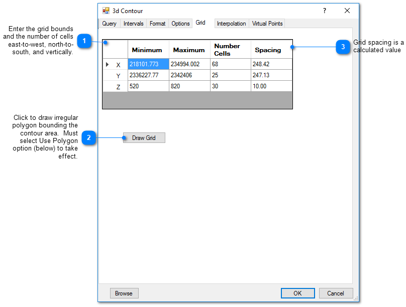
Grid Tab
This tab allows the user to define the grid on which the measured values will be interpolated prior to contouring. Increasing the number of cells may improve the faithfulness of the contoured result to the interpolated field, but increases the time to generate the contours.
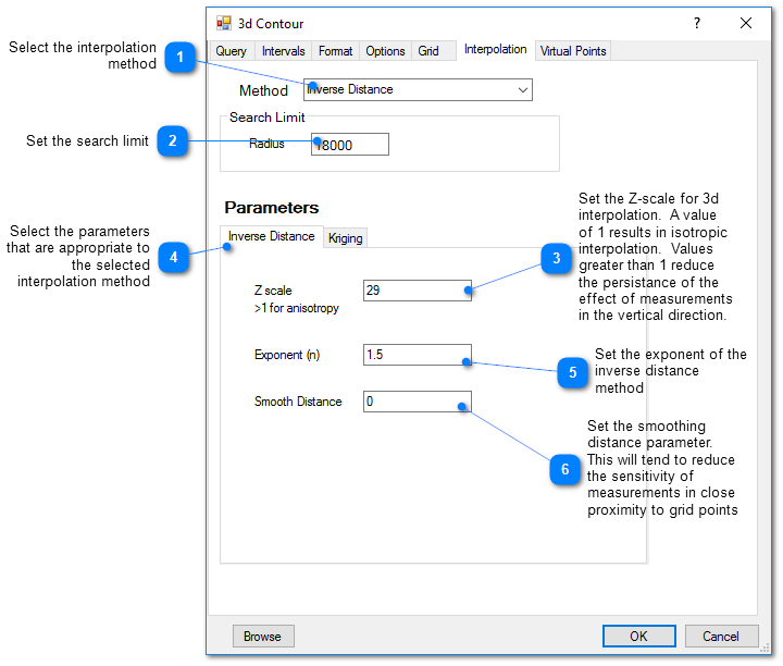
This tab allows the user to select the interpolation scheme and the parameters of the interpolation method. The correct selection of interpolation parameters is critical to generate contours that accurately reflect the field data and our expectations of how the values vary between the measured data points. The default parameters are frequently adequate, although some improvement can be anticipated through trial and error. There is no single, objectively optimal set of interpolation parameters. Different methods and parameters work best for different data sets.
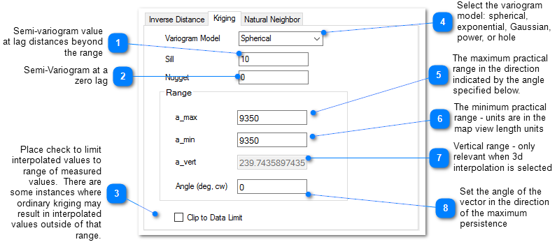
Kriging Parameter
The kriging routines are derived from the kt3d routine of the Geostatistical Software Library (GSLIB) authored by Clayton Deutsch and Andre Journel.
The reference GSLIB: Geostatistical Software Library and Users' Guide is highly recommended. The following equations are the spherical semivariogram models used by EnviroInsite for an isotropic system, where h is the lag, c is the sill, and a is the (practical) range.
(Source: Introduction to Geostatistics and Variogram Analysis, available here).
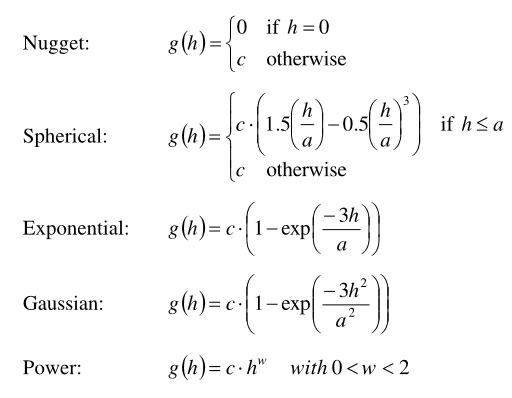
For anisotrophic systems, h/a in the previous is calculated as
![]()
Inverse Distance Parameters
Z Scale – The vertical distances between a measured value and a grid node are multiplied by this value prior to calculating the interpolation weight assigned to a measured value. Thus, points not aligned horizontally are effectively further apart by a factor equivalent to the Z scale. Z scale values greater than one will result in lower weights assigned to measured values that are not at the same elevation as the grid point.
Exponent – The measured values are assigned weights that are equal to one over the distance between the measured value and the grid point raised to some power. This exponent is the power used in that calculation.
Smooth Distance – The inverse distance method tends to cause a kind of bubbly surface with the bubbles coinciding with measurement points. This type of trend can be reduced by introducing a non-zero smoothing distance. The smoothing distance is effected by adding this distance to the separation distance between the measurement point and the grid point prior to calculating the interpolation weight. This effectively diminishes the weight assigned to points at distances close to the Smooth-Distance, while not appreciably impacting the calculated weights for more distant points.
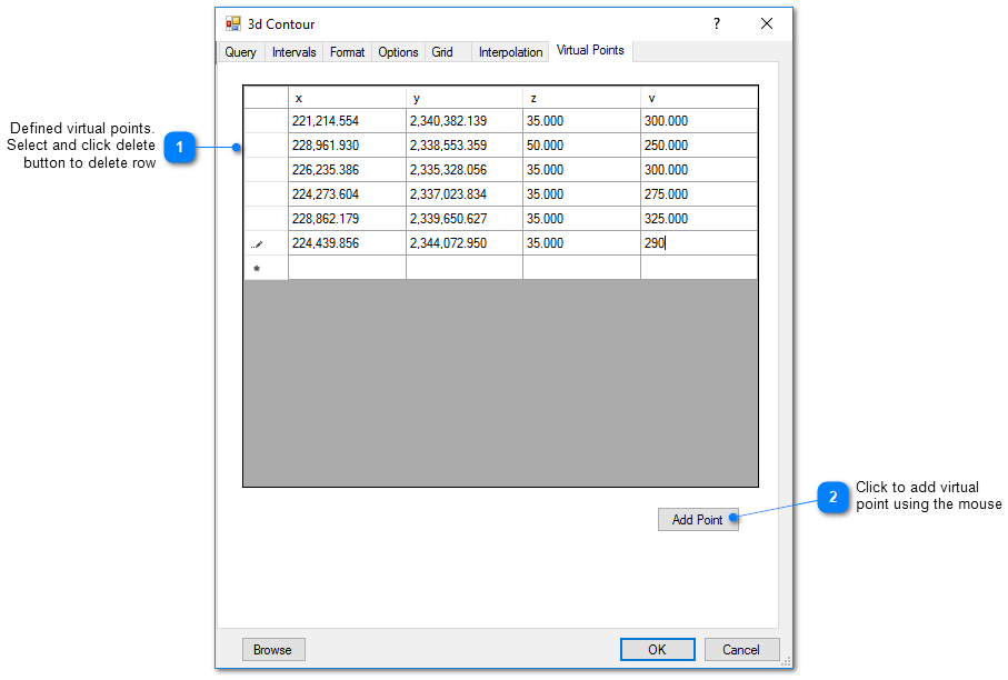
Virtual Points Tab
Virtual points are used to control the generation of contours with sparse data. In those cases or in cases of water bodies that are hydraulically continuous with groundwater, it may be advantageous to create virtual measurement points that will control the resulting contours.