Gradient arrows plot the direction of descent of the user-selected field. In most cases, the selected field is the water table elevation and the gradient arrows depict the direction of flow. In constructing the plot, the user specifies a rectangular domain and divides the space into a set of cells making up a rectangular grid. The field values are interpolated to the mid-points of the lines bordering each cell and the gradient is calculated by subtracting the difference in value across the cell by the cell width or height.
Prior to generating gradient, develop an appropriate 2D surface. Use the same grid and interpolation method /parameters for both the 2D contours and the gradient arrows.
Click Plot> 2D Data from the main menu and select Gradient. The Gradient dialog box opens. Modify the gradient properties on the Query tab, Format tab, Grid tab, Interpolation tab, Legend tab, Virtual Points tab, and EQuIS Query tab as desired. Click the OK button to save changes.
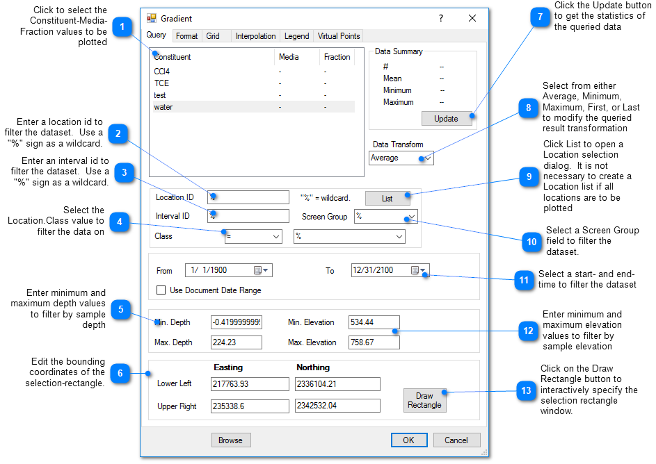
Query Tab
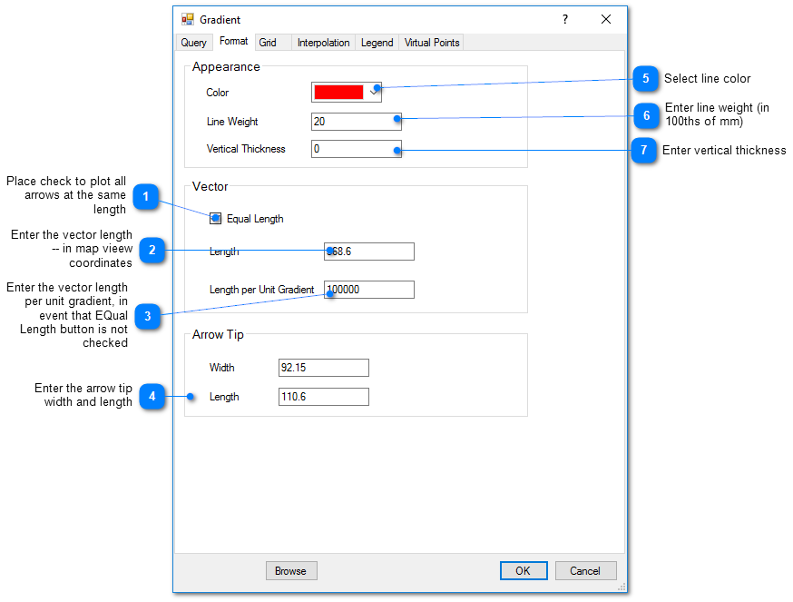
Format Tab
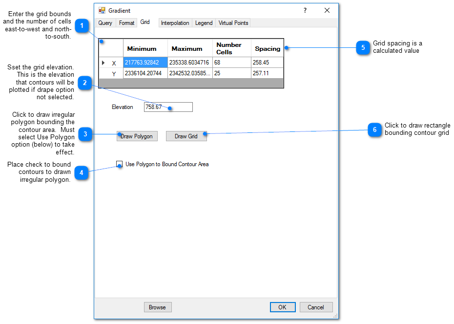
Grid Tab
This tab allows the user to define the grid on which the measured values will be interpolated prior to contouring. Increasing the number of cells may improve the faithfulness of the contoured result to the interpolated field, but increases the time to generate the contours.
Interpolation Tab
This tab allows the user to select the interpolation scheme and the parameters of the interpolation method. The correct selection of interpolation parameters is critical for generation of contours that accurately reflect the field data and our expectations of how the values vary between the measured data points. The default parameters are frequently adequate, although some improvement can be anticipated through trial and error.
Method – Select the contouring method from inverse distance, kriging, natural neighbor, and triangulation.
Search Limit Radius – The cutoff distance establishes the maximum distance from the interpolated point for which a measured value will be used in the interpolation function. Used by both kriging and inverse distance routines.
Kriging Parameters
The kriging routines are derived from the kt3d routine of the Geostatistical Software Library (GSLIB) authored by Clayton Deutsch and Andre Journel.
Variogram Model – Select from the spherical, exponential, gaussian, power, and hole variogram models using conventions of GSLIB.
Sill – Set the variogram model sill or c value.
Nugget – Set local scale variability.
Range a max – Set maximum horizontal range.
Range a min – Set minimum horizontal range.
Range a vert – Set vertical range.
Angle – Rotation angle in degrees clockwise about 12 o'clock of axis defining the direction of maximum horizontal range. In some cases it may be advantageous to increase the a max value and to align this axis with the direction of ground-water flow.
Inverse Distance Parameters
Z Scale – The vertical distances are multiplied by this value prior to calculating the interpolation weight assigned to a measured value. Z Scale values greater than one will result in lower weights assigned to measured values that are not at the same elevation as the grid point.
Exponent – The measured values are assigned weights that are equal to one over the distance between the measured value and the grid point raised to some power. This exponent is the power used in that calculation.
Smooth Distance – The inverse distance method tends to cause a kind of bubbly surface with the bubbles coinciding with measurement points. This type of trend can be reduced by introducing a non-zero smoothing distance. The smoothing distance is effected by adding this distance to the separation distance between the measurement point and the grid point prior to calculating the interpolation weight.
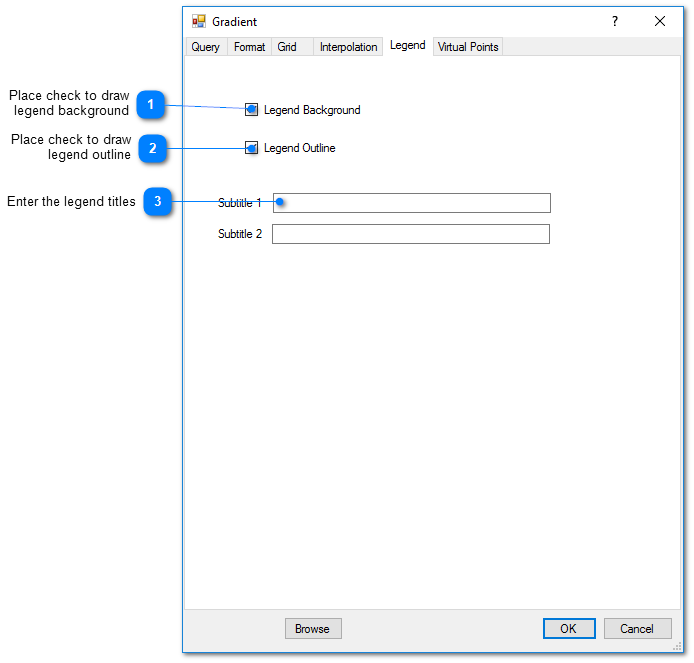
Legend Tab
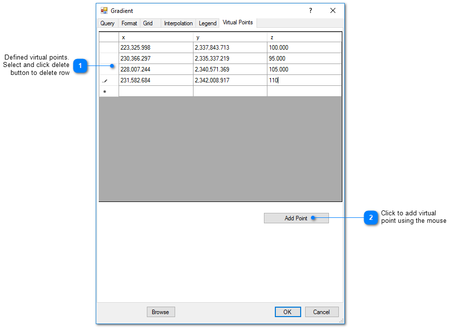
Virtual Points Tab
Virtual points are used to control the generation of gradient arrows in areas with sparse data. In those cases, it may be advantageous to create virtual measurement points that will control the resulting gradient arrows.