This exercise demonstrates how to use EQuIS Data Processor (EDP) or EDGE to calculate instant flow in a river or stream from field measurements, based on the Flow Curve method.
The calculation can be performed by use of one of two equations:
Equation A. i) ‘Standard Method’: X = (gauge/a)^(1/b)
Equation A. ii) ‘Intercept Method’: X = a * (gauge-c)^b
where: X = instant flow (m3/sec)
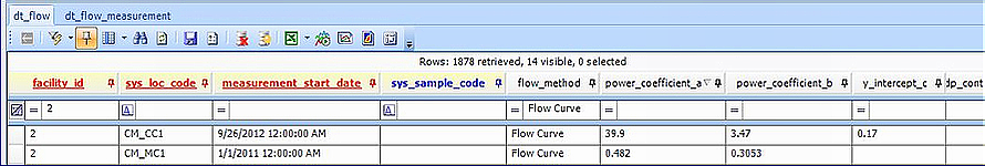
a = dt_flow.power_coefficient_a
b = dt_flow.power_coefficient_b
c = dt_flow.y_intercept_c (this is the field gauge reading at 'zero' flow, i.e. ground level) (m)
gauge = dt_flow.gauge - the staff field gauge reading within the water body (m)
Power coefficients ‘a’ and ‘b’ are specific to each stream measurement location or SYS_LOC_CODE. These values will need to be calculated using actual measurements of flow velocity and staff gauge height readings collected over a period of time plotted as a ‘gauge-flow’ (stage-discharge) plot.
The instant calculation in EDGE or EDP will be performed using the most recent power coefficients for a SYS_LOC_CODE in DT_FLOW. The coefficient values can be added to a record which has an instant_flow value, for reference. The values entered here will not change the calculated value.
The Equation A. i) ‘Standard Method’ will be used where there is no value for ‘c’ (intercept) entered in DT_FLOW. Where a value for ‘c’ is entered in DT_FLOW, then the Equation A. ii) ‘Intercept Method’ will be used.
Follow these steps to perform the instant flow calculation:
1.Open EQuIS Professional.
2.Open data table DT_FLOW.
3.Create a new row for the SYS_LOC_CODE and enter the pre-determined values for POWER_COEFFICIENT_A and POWER_COEFFICIENT_B. If the SYS_LOC_CODE also has a value for Y_INTERCEPT_C, then this should also be entered. If there is no value for Y_INTERCEPT_C (i.e. the staff gauge is set at 0m at ground level), then leave this column blank.
4.Enter the FLOW_METHOD as ‘flow curve'.
5.When creating an EDD with the flow information using the EDGE Field EDD, be sure to add a check to "Flow parameters".
Note: The presence or absence of a value for Y_INTERCEPT_C’ will determine which instant flow equation is used. |
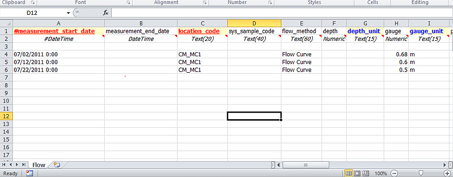
6.Open the field flow EDD, either in the field via EDGE, or in Excel.
7.Enter the field staff gauge readings in the ‘Flow’ tab of the EDD.
8.Enter the FLOW_METHOD in the EDD as ‘flow curve’.
9.In EDGE, select the FLOW_METHOD as FLOW CURVE from the drop-down menu. Required fields are MEASUREMENT_START_DATE and LOCATION_CODE’ (this synonymous with SYS_LOC_CODE). In order for the calculation to run, the GAUGE column must be populated (as well as the power coefficients in DT_FLOW). Make sure all titles for EDDs, etc., are in the correct format. Save the EDD.

10.If using EDGE, on entering the GAUGE data in EDGE, the INSTANT_FLOW column should populate automatically.
11.If using an EDD in Excel, open EQuIS Data Processor (EDP) and select the desired format. Click on ‘EDD’ in the ‘Open’ menu and select the EDD for upload.
EDP Import with Flow Calculation Completed
When the EDD is opened, EDP will perform the instant flow calculation, and the columns INSTANT_FLOW and INSTANT_FLOW_UNIT will be populated. The REMARKS column (last column in the EDD), will be populated with ‘EDP populated instant_flow’ to confirm this. The data can then be ‘created’ and ‘committed’, which will populate the INSTANT_FLOW and INSTANT_FLOW_UNIT columns within DT_FLOW. During the Create step, a record will also be created in DT_SAMPLE and DT_FIELD_SAMPLE.