EnviroInsite provides the capacity to contour stratigraphy depth, elevation, and thickness. The contouring routines provide the same features as for the contouring of measured water levels or concentrations.
Click Plot> Stratigraphy from the main menu and select Contours. The Contour Stratigraphy dialog box opens. Modify the contour properties on the Query tab, Interval tab, Format tab, Options tab, Grid tab, Interpolation tab, Virtual Points tab, and EQuIS Query tab as desired. Click the OK button to save changes.
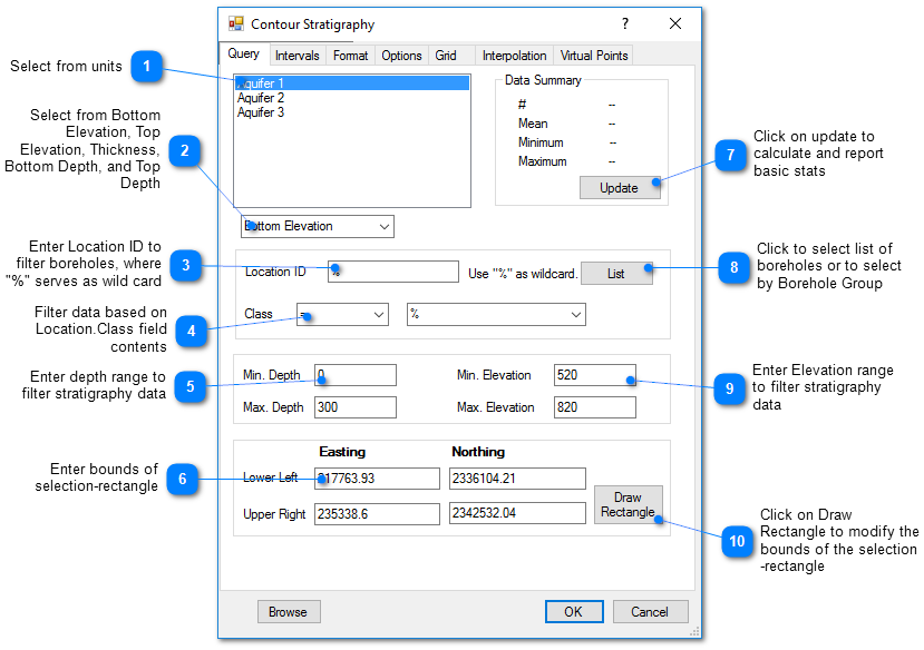
Query Tab
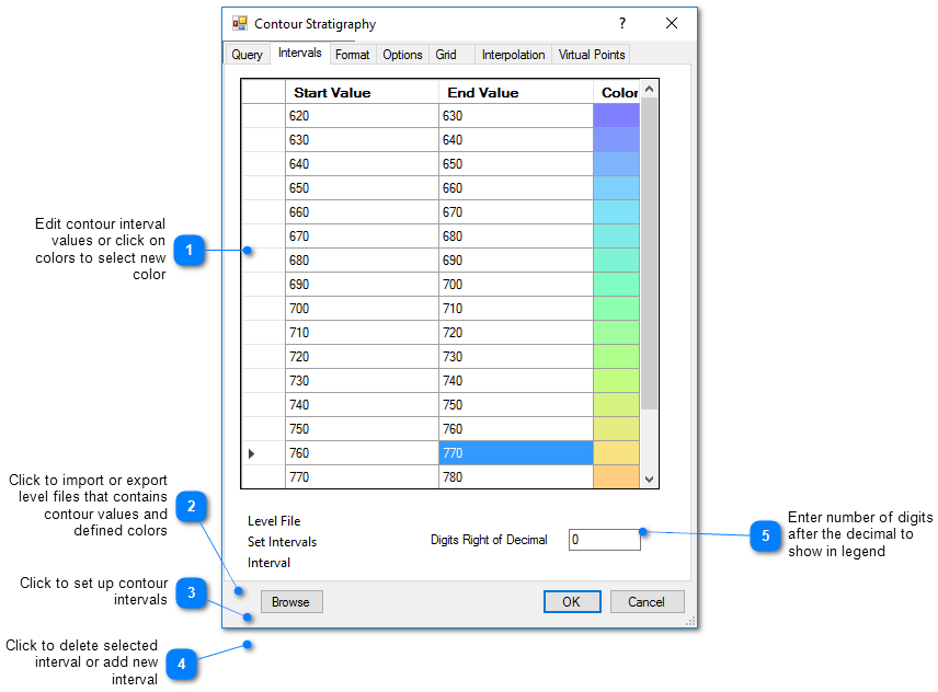
Intervals Tab
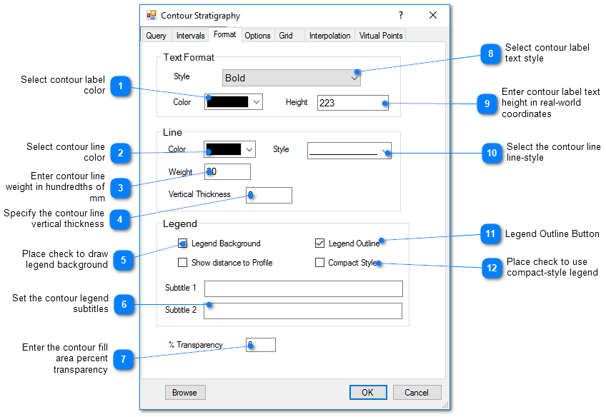
Format Tab
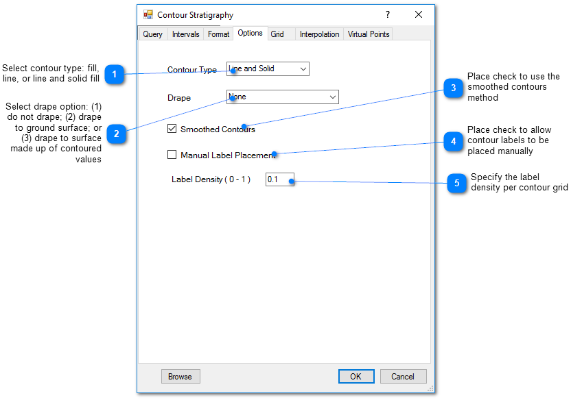
Options Tab
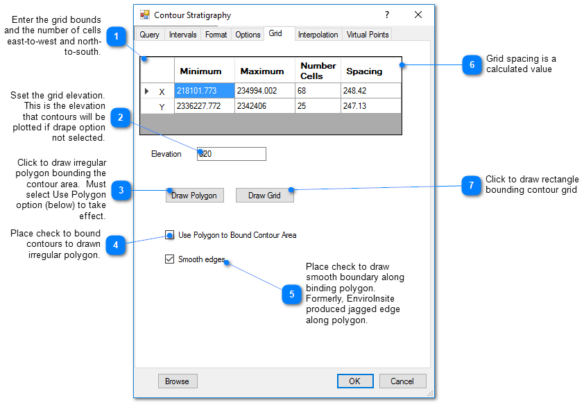
Grid Tab
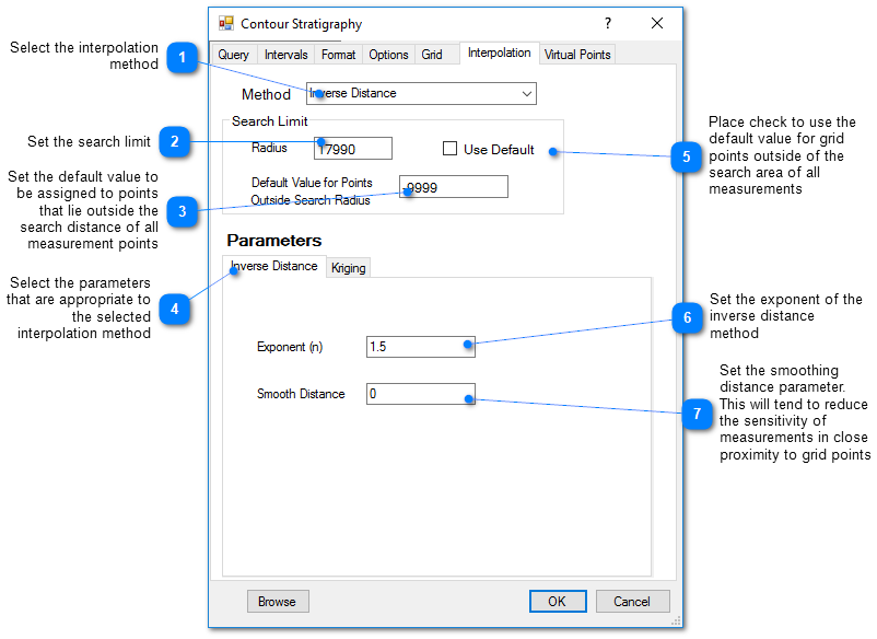
Interpolation Tab
This tab allows the user to select the interpolation scheme and the parameters of the interpolation method. The correct selection of interpolation parameters is critical to generate contours that accurately reflect the field data and our expectations of how the values vary between the measured data points. The default parameters are frequently adequate, although some improvement can be anticipated through trial and error. There is no single, objectively optimal set of interpolation parameters. Different methods and parameters work best for different data sets.
Kriging Parameters
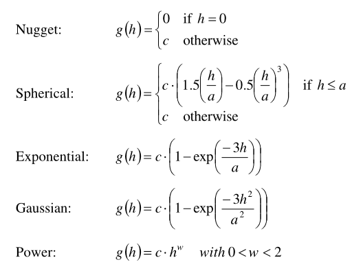
The kriging routines are derived from the kt3d routine of the Geostatistical Software Library (GSLIB) authored by Clayton Deutsch and Andre Journel.
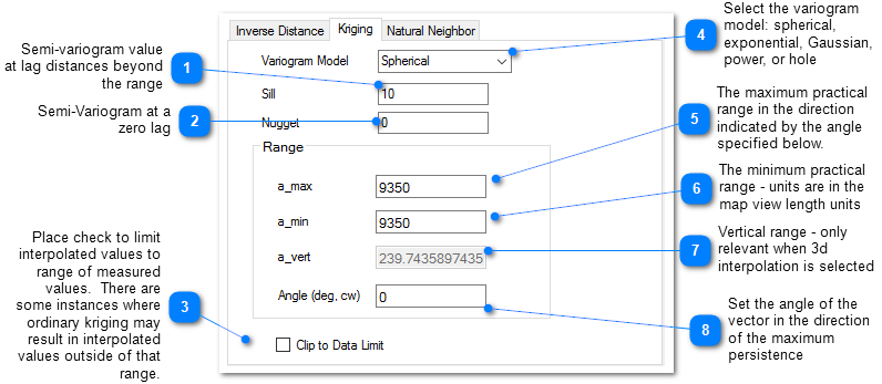
The reference GSLIB: Geostatistical Software Library and Users' Guide is highly recommended. The following equations are the spherical semivariogram models used by EnviroInsite for an isotropic system, where h is the lag, c is the sill, and a is the (practical) range.
(Source: Introduction to Geostatistics and Variogram Analysis, available here).
For anisotropic systems, h/a in the previous is calculated as
![]()
Inverse Distance Parameters
Exponent – The measured values are assigned weights that are equal to one over the distance between the measured value and the grid point raised to some power. This exponent is the power used in that calculation.
Smooth Distance – The inverse distance method tends to cause a kind of bubbly surface with the bubbles coinciding with measurement points. This type of trend can be reduced by introducing a non-zero smoothing distance. The smoothing distance is effected by adding this distance to the separation distance between the measurement point and the grid point prior to calculating the interpolation weight. This effectively diminishes the weight assigned to points at distances close to the Smooth-Distance, while not appreciably impacting the calculated weights for more distant points.
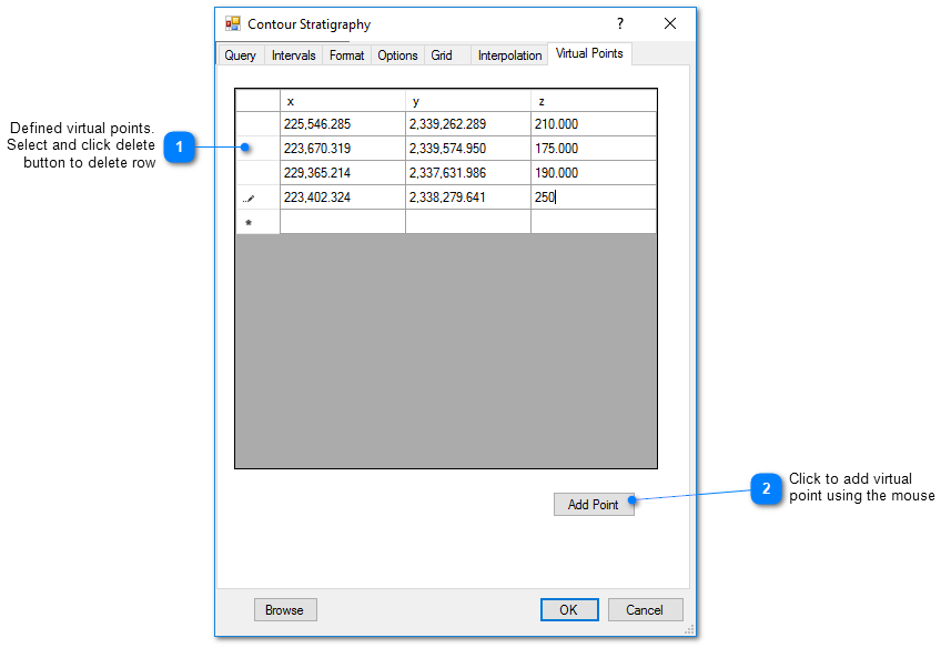
Virtual Points Tab
Virtual points are used to control the generation of contours with sparse data. In those cases, it may be advantageous to create virtual measurement points that will control the resulting contours.