The standard method for contouring involves the interpolation of measured values onto a rectangular mesh and contouring of the gridded data. Inverse distance, kriging, and natural neighbor are offered as interpolation methods. Contours are constructed using either the xfarbe routines (Algorithm 671 - FARB-E-2D: Fill Area with Bicubics on Rectangles, ACM Transactions on Mathematical Software, vol. 15, no. 1, March 1989) or a 2D version of the marching cubes algorithm. For contours generated on a vertical profile, the interpolation is performed in three dimensions to obtain the data values on a three-dimensional grid. In plan mode, the interpolation procedure does not consider the elevation or depth of a particular measurement in its interpolation onto the rectangular mesh corner points, although data queries can exclude source data measurements by depth or elevation. For example, to contour only shallow measurements, set the depth or elevation query to select only those measurements.
An alternative triangulation contouring procedure is available for plan view contours. This involves the generation of triangles, with corners at the location of the measured data points. The contours are constructed within each triangle based on linear interpolation and the values of the contoured data at the corner nodes. This method is frequently useful for data reported on a rectangular grid.
EnviroInsite Videos
•View a training video on 2D contouring in EnviroInsite here.
•View a training video on contouring using the inverse distance interpolation method in EnviroInsite here.
•View a training video on contouring using the kriging interpolation method in EnviroInsite here.
Contouring Tips
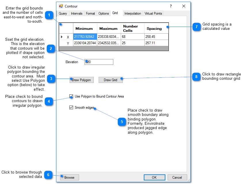
Confine the area for contouring to the data extent. Go to the Grid tab within the Contour dialog box and select the Draw Grid button or the Draw Polygon button. Draw a rectangle or shape that excludes areas beyond the extent of the data.
For contouring values that vary over several orders of magnitude, select Log Transform on the Options tab of the Contour dialog box. This interpolate on the log of the values rather than the actual values. The effect reduces the spread of the contours away from the peak values.
Use the kriging interpolation option. In many cases, the inverse distance interpolation will create a kind of bubbly effect around the data points. Natural neighbor depends on triangulation and can be problematic contouring to the edge of the data or beyond.
Adjust the kriging interpolation range values to a distance for which you want the measured values to have an impact on the contours. For example, if high interpolation values extend a great distance from a peak measurement location, reduce the range value to limit the influence of the peak measurement on the contours. Reducing the search radius may have the same impact as reducing the range, but may cause the results to be non-smooth.
If the direction of flow is known, you may want to elongate the persistence of interpolated values in the direction of flow. Do this by selecting the kriging interpolation option and adjusting the maximum range. Set the maximum range angle to be aligned with the direction of groundwater flow. The angle is specified in degrees clockwise relative to due north.
Creating a Contour Plot
Click Plot> 2D Data from the main menu and select Contours. The Contour dialog box opens. Modify the contour properties on the Query tab, Interval tab, Format tab, Options tab, Grid tab, Interpolation tab, Virtual Points tab, and EQuIS Query tab as desired. Click the OK button to save changes.
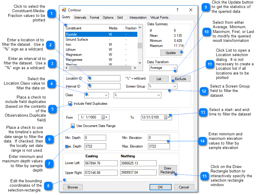
Query Tab
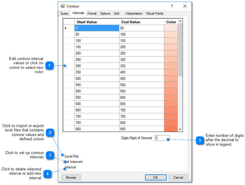
Intervals Tab
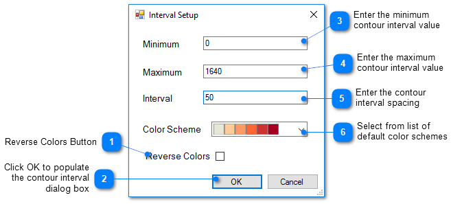
Interval Setup
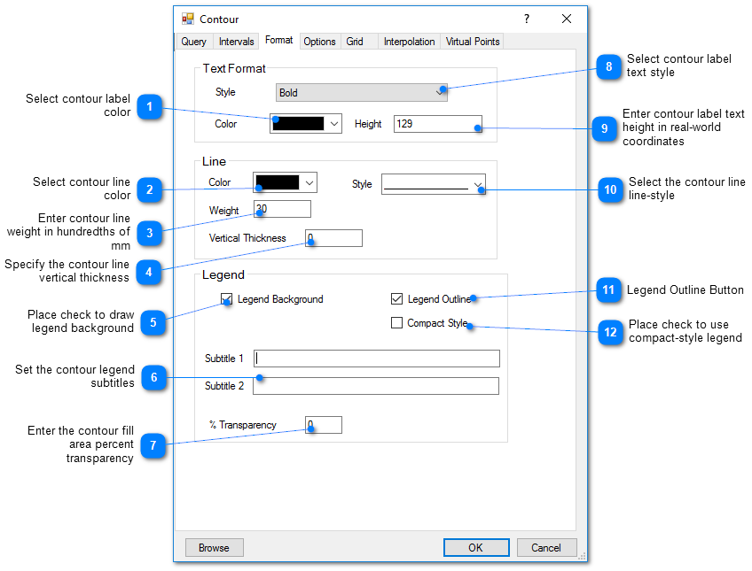
Format Tab
Options Tab
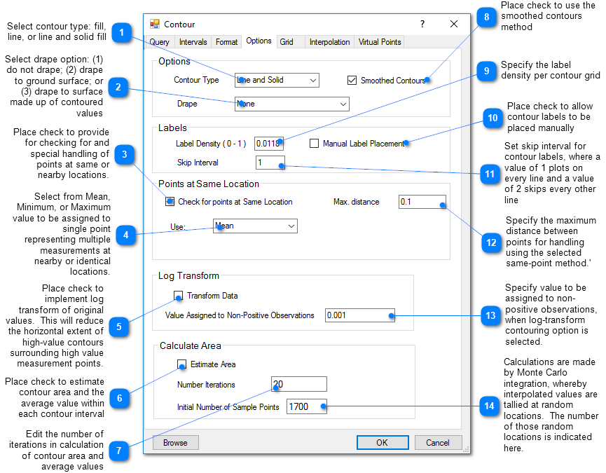
Estimate Area
In many cases, there is only one measurement at each location. Therefore, estimates of contaminant mass or the volume with concentrations exceeding some value will need to be made using a presumed contaminant thickness. Place a check in the Estimate Area box. The results (contour interval, average value, area) are written out to the Data tab in the Work Log window. Copy and paste the final result from the Data tab to Excel and set up the calculations in Excel for some assumed finite contaminated thickness. The mass associated with each interval is the product of the average value, the area, and the thickness. If this is a dissolved constituent, then you also need to multiply by the porosity. You may also want to account for an adsorbed phase by multiplying by the retardation factor. If there are multiple concentration measurements at different elevations, then you may want to select Check for Points at Same Location and select the Maximum value.
Grid Tab
This tab allows the user to define the grid on which the measured values will be interpolated prior to contouring. Increasing the number of cells may improve the faithfulness of the contoured result to the interpolated field, but increases the time to generate the contours.
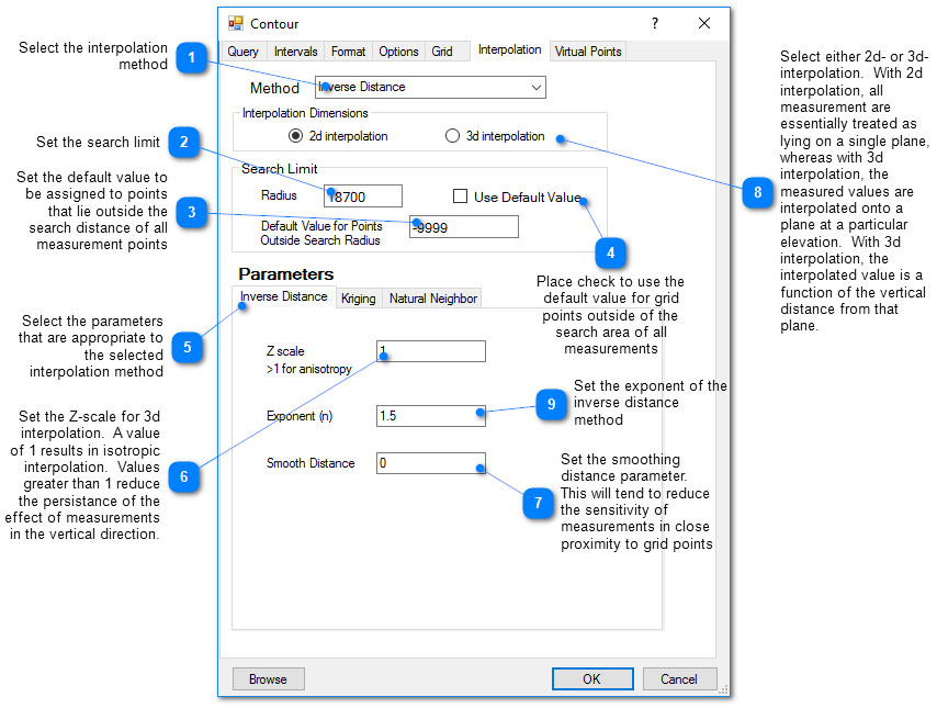
Interpolation Tab
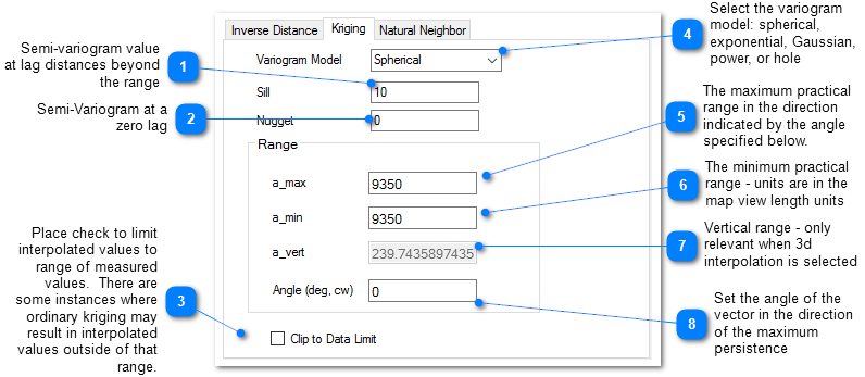
This tab allows the user to select the interpolation scheme and the parameters of the interpolation method. The correct selection of interpolation parameters is critical to generate contours that accurately reflect the field data and our expectations of how the values vary between the measured data points. The default parameters are frequently adequate, although some improvement can be anticipated through trial and error. There is no single, objectively optimal set of interpolation parameters. Different methods and parameters work best for different data sets.
Kriging Parameters
The kriging routines are derived from the kt3d routine of the Geostatistical Software Library (GSLIB) authored by Clayton Deutsch and Andre Journel.
The reference GSLIB: Geostatistical Software Library and Users' Guide is highly recommended. The following equations are the spherical semivariogram models used by EnviroInsite for an isotropic system, where h is the lag, c is the sill, and a is the (practical) range.
(Source: Introduction to Geostatistics and Variogram Analysis, available here).
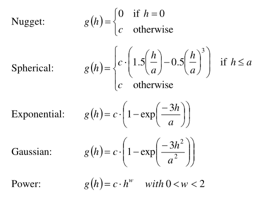
For anisotropic systems, h/a in the previous is calculated as
![]()
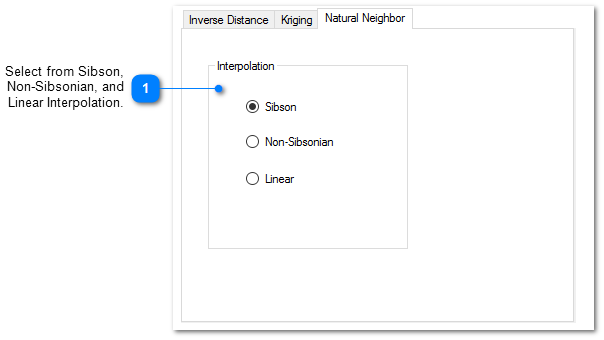
Natural Neighbor Parameters
The natural neighbor interpolation makes use of an adapted version of the public domain natural neighbor code developed by Pavel Sakov of CSIRO Marine Research.
Inverse Distance Parameters
Z Scale – The vertical distances between a measured value and a grid node are multiplied by this value prior to calculating the interpolation weight assigned to a measured value. Thus, points not aligned horizontally are effectively further apart by a factor equivalent to the Z scale. Z scale values greater than one will result in lower weights assigned to measured values that are not at the same elevation as the grid point.
Exponent – The measured values are assigned weights that are equal to one over the distance between the measured value and the grid point raised to some power. This exponent is the power used in that calculation.
Smooth Distance – The inverse distance method tends to cause a kind of bubbly surface with the bubbles coinciding with measurement points. This type of trend can be reduced by introducing a non-zero smoothing distance. The smoothing distance is effected by adding this distance to the separation distance between the measurement point and the grid point prior to calculating the interpolation weight. This effectively diminishes the weight assigned to points at distances close to the Smooth-Distance, while not appreciably impacting the calculated weights for more distant points.
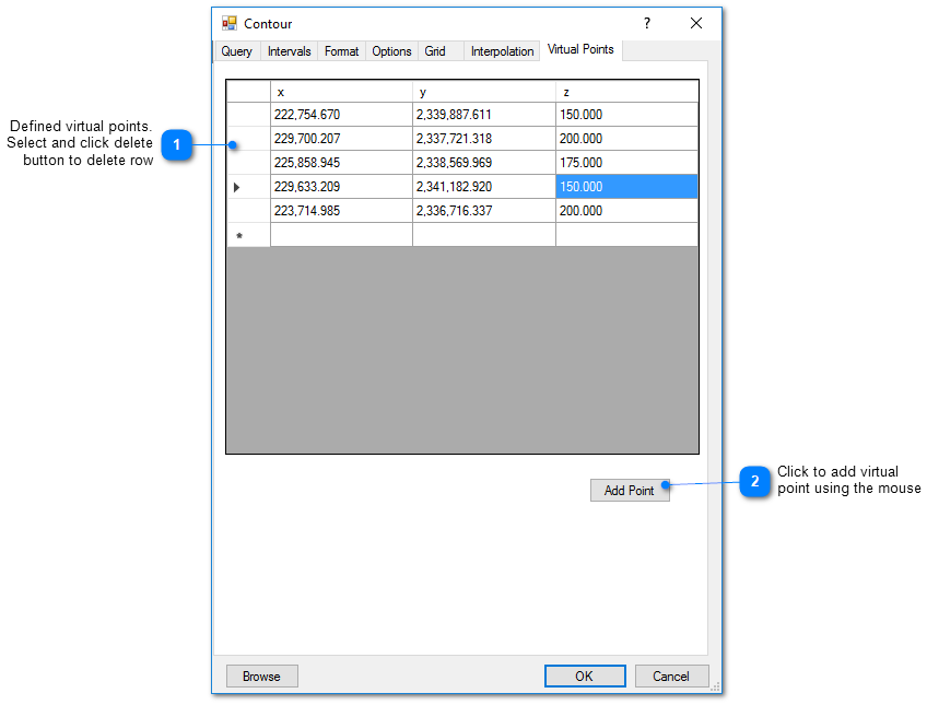
Virtual Points Tab
Virtual points are used to control generating contours with sparse data. In those cases or in cases of water bodies that are hydraulically continuous with groundwater, it may be advantageous to create virtual measurement points that will control the resulting contours.